Part 1

Previously we’ve seen some of the very basic image analysis operations in Python. In this last part of basic image analysis, we’ll go through some of the following contents.

Following contents is the reflection of my completed academic image processing course in the previous term. So, I am not planning on putting anything into production sphere. Instead, the aim of this article is to try and realize the fundamentals of a few basic image processing techniques. For this reason, I am going to stick to using imageio or numpy mainly to perform most of the manipulations, although I will use other libraries now and then rather than using most wanted tools such as OpenCV :

In the previous article, we’ve gone through some of the following basic operations. To keep pace with today’s content, continuous reading is highly appreciated.

• Importing images and observe it’s properties
• Splitting the layers
• Greyscale
• Using Logical Operator on pixel values
• Masking using Logical Operator
• Satellite Image Data Analysis

Table of Contents

• Intensity Transformation
• Convolution
• Segmentation
  • Thresholding
  • Object Detection
• Vectorization
  • Contour tracking
• Image Compression
  • Stacked Autoencoder

I’m so excited, let’s begin.

Intensity Transformation

Let’s begin with importing an image.

%matplotlib inline

import imageio
import matplotlib.pyplot as plt
import warnings
import matplotlib.cbook
warnings.filterwarnings("ignore",category=matplotlib.cbook.mplDeprecation)

pic = imageio.imread('img/parrot.jpg')

plt.figure(figsize = (6,6))
plt.imshow(pic);
plt.axis('off');

Image Negative

The intensity transformation function mathematically defined as:

$s = T ( r )$

where $r$ is the pixels of the input image and $s$ is the pixels of the output image. $T$ is a transformation function that maps each value of $r$ to each value of $s$.

Negative transformation, which is the invert of identity transformation. In negative transformation, each value of the input image is subtracted from the $L-1$ and mapped onto the output image.

In this case, the following transition has been done.

$s = (L – 1) – r$

So each value is subtracted by 255. So what happens is that the lighter pixels become dark and the darker picture becomes light. And it results in image negative.

negative = 255 - pic # neg = (L-1) - img

plt.figure(figsize = (6,6))
plt.imshow(negative);
plt.axis('off');

Resources:

• 1 - 2

Log transformation

The log transformations can be defined by this formula

$s = c * log(r + 1)$

Where $s$ and $r$ are the pixel values of the output and the input image and $c$ is a constant. The value 1 is added to each of the pixel value of the input image because if there is a pixel intensity of 0 in the image, then $log (0)$ is equal to infinity. So 1 is added, to make the minimum value at least 1.

During log transformation, the dark pixels in an image are expanded as compared to the higher pixel values. The higher pixel values are kind of compressed in log transformation. This result in the following image enhancement.

The value of $c$ in the log transform adjust the kind of enhancement we are looking for.

%matplotlib inline

import imageio
import numpy as np
import matplotlib.pyplot as plt

pic = imageio.imread('img/parrot.jpg')
gray = lambda rgb : np.dot(rgb[... , :3] , [0.299 , 0.587, 0.114]) 
gray = gray(pic)

'''
log transform
-> s = c*log(1+r)

So, we calculate constant c to estimate s
-> c = (L-1)/log(1+|I_max|)

'''

max_ = np.max(gray)

def log_transform():
    return (255/np.log(1+max_)) * np.log(1+gray)

plt.figure(figsize = (5,5))
plt.imshow(log_transform(), cmap = plt.get_cmap(name = 'gray'))
plt.axis('off');

Resources:

• 1 - 2

Gamma Correction

Gamma correction, or often simply gamma, is a nonlinear operation used to encode and decode luminance or tristimulus values in video or still image systems. Gamma correction is also known as the Power Law Transform. First, our image pixel intensities must be scaled from the range 0, 255 to 0, 1.0. From there, we obtain our output gamma corrected image by applying the following equation:

$V_o = V_i^\frac{1}{G}$

Where $V_i$ is our input image and G is our gamma value. The output image, $V_o$ is then scaled back to the range 0-255.

A gamma value, G < 1 is sometimes called an encoding gamma, and the process of encoding with this compressive power-law nonlinearity is called gamma compression; Gamma values < 1 will shift the image towards the darker end of the spectrum.

Conversely, a gamma value G > 1 is called a decoding gamma and the application of the expansive power-law nonlinearity is called gamma expansion. Gamma values > 1 will make the image appear lighter. A gamma value of G = 1 will have no effect on the input image:

import imageio
import matplotlib.pyplot as plt

# Gamma encoding 
pic = imageio.imread('img/parrot.jpg')
gamma = 2.2 # Gamma < 1 ~ Dark  ;  Gamma > 1 ~ Bright

gamma_correction = ((pic/255) ** (1/gamma)) 
plt.figure(figsize = (5,5))
plt.imshow(gamma_correction)
plt.axis('off');

The Reason of Gamma Correction

The reason we apply gamma correction is that our eyes perceive color and luminance differently than the sensors in a digital camera. When a sensor on a digital camera picks up twice the amount of photons, the signal is doubled. However, our eyes do not work like this. Instead, our eyes perceive double the amount of light as only a fraction brighter. Thus, while a digital camera has a linear relationship between brightness our eyes have a non-linear relationship. In order to account for this relationship, we apply gamma correction.

There is some other linear transformation function. Listed below:

• Contrast Stretching
• Intensity-Level Slicing
• Bit-Plane Slicing

Resources:

• 1 - 2 - 3 - 4

Convolution

We’ve discussed briefly in our previous article is that, when a computer sees an image, it sees an array of pixel values. Now, Depending on the resolution and size of the image, it will see a 32 x 32 x 3 array of numbers where the 3 refers to RGB values or channels. Just to drive home the point, let’s say we have a color image in PNG form and its size is 480 x 480. The representative array will be 480 x 480 x 3. Each of these numbers is given a value from 0 to 255 which describes the pixel intensity at that point.

Like we mentioned before, the input is a 32 x 32 x 3 array of pixel values. Now, the best way to explain a convolution is to imagine a flashlight that is shining over the top left of the image. Let’s say that the flashlight shines covers a 3 x 3 area. And now, let’s imagine this flashlight sliding across all the areas of the input image. In machine learning terms, this flashlight is called a filter or kernel or sometimes referred to as weights or mask and the region that it is shining over is called the receptive field.

Now, this filter is also an array of numbers where the numbers are called weights or parameters. A very important note is that the depth of this filter has to be the same as the depth of the input, so the dimensions of this filter are 3 x 3 x 3.

An image kernel or filter is a small matrix used to apply effects like the ones we might find in Photoshop or Gimp, such as blurring, sharpening, outlining or embossing. They’re also used in machine learning for feature extraction, a technique for determining the most important portions of an image. For more, have a look at Gimp’s excellent documentation on using Image kernel’s. We can find a list of most common kernels here.

Now, let’s take the filter to the top left corner. As the filter is sliding, or convolving, around the input image, it is multiplying the values in the filter with the original pixel values of the image (aka computing element-wise multiplications). These multiplications are all summed up. So now we have a single number. Remember, this number is just representative of when the filter is at the top left of the image. Now, we repeat this process for every location on the input volume. Next step would be moving the filter to the right by a stride or step 1 unit, then right again by stride 1, and so on. Every unique location on the input volume produces a number. We can also choose stride or the step size 2 or more, but we have to care whether it will fit or not on the input image.

After sliding the filter over all the locations, we will find out that, what we’re left with is a 30 x 30 x 1 array of numbers, which we call an activation map or feature map. The reason we get a 30 x 30 array is that there are 900 different locations that a 3 x 3 filter can fit on a 32 x 32 input image. These 900 numbers are mapped to a 30 x 30 array. We can calculate the convolved image by following:

\begin{align} Convolved: \frac{N - F}{S} + 1 \end{align}

where $N$ and $F$ represent Input image size and kernel size respectively and $S$ represent stride or step size. So, in this case, the output would be

\begin{align} \frac{32 - 3}{1} + 1 &= 30 \end{align}

Let’s say we’ve got a following $3x3$ filter, convolving on a $5x5$ matrix and according to the equation we should get a $3x3$ matrix, technically called activation map or feature map.

let’s take a look visually,

Moreover, we practically use more filters instead of one. Then our output volume would be $28 x 28 x n$ (where n is the number of activation map). By using more filters, we are able to preserve the spatial dimensions better.

However, For the pixels on the border of the image matrix, some elements of the kernel might stand out of the image matrix and therefore does not have any corresponding element from the image matrix. In this case, we can eliminate the convolution operation for these positions which end up an output matrix smaller than the input or we can apply padding to the input matrix.

Now, I do realize that some of these topics are quite complex and could be made in whole posts by themselves. In an effort to remain concise yet retain comprehensiveness, I will provide links to resources where the topic is explained in more detail.

Let’s first apply some custom uniform window to the image. This has the effect of burning the image, by averaging each pixel with those nearby

%%time
import numpy as np
import imageio
import matplotlib.pyplot as plt
from scipy.signal import convolve2d

def Convolution(image, kernel):
    conv_bucket = []
    for d in range(image.ndim):
        conv_channel = convolve2d(image[:,:,d], kernel, 
                               mode="same", boundary="symm")
        conv_bucket.append(conv_channel)
    return np.stack(conv_bucket, axis=2).astype("uint8")


kernel_sizes = [9,15,30,60]
fig, axs = plt.subplots(nrows = 1, ncols = len(kernel_sizes), figsize=(15,15));

pic = imageio.imread('img:/parrot.jpg')

for k, ax in zip(kernel_sizes, axs):
    kernel = np.ones((k,k))
    kernel /= np.sum(kernel)
    ax.imshow(Convolution(pic, kernel));
    ax.set_title("Convolved By Kernel: {}".format(k));
    ax.set_axis_off();

Depending on the element values, a kernel can cause a wide range of effects. Check out this site to visualize the output of various kernel. In this article, we’ll go through few of them.

Following is an Outline Kernel. An outline kernel (aka “edge” kernel) is used to highlight large differences in pixel values. A pixel next to neighbor pixels with close to the same intensity will appear black in the new image while one next to neighbor pixels that differ strongly will appear white.

%%time
from skimage import color
from skimage import exposure
import numpy as np
import imageio
import matplotlib.pyplot as plt 

# import image
pic = imageio.imread('img/crazycat.jpeg')
plt.figure(figsize = (5,5))
plt.imshow(pic)
plt.axis('off');

# Convert the image to grayscale 
img = color.rgb2gray(pic)

# outline kernel - used for edge detection
kernel = np.array([[-1,-1,-1],
                   [-1,8,-1],
                   [-1,-1,-1]])

# we use 'valid' which means we do not add zero padding to our image
edges = convolve2d(img, kernel, mode = 'valid')


# Adjust the contrast of the filtered image by applying Histogram Equalization
edges_equalized = exposure.equalize_adapthist(edges/np.max(np.abs(edges)),
                                              clip_limit = 0.03)

# plot the edges_clipped
plt.figure(figsize = (5,5))
plt.imshow(edges_equalized, cmap='gray')    
plt.axis('off');

Let’s play around for a while with different types of other filters. Let’s choose with Sharpen Kernel. The Sharpen Kernel emphasizes differences in adjacent pixel values. This makes the image look more vivid.

Let’s apply the edge detection kernel to the output of the sharpen kernel and also further normalizing with box blur filter.

%%time

from skimage import color
from skimage import exposure
from scipy.signal import convolve2d
import numpy as np
import imageio
import matplotlib.pyplot as plt 

# Convert the image to grayscale
img = color.rgb2gray(pic)  

# apply sharpen filter to the original image
sharpen_kernel = np.array([[0,-1,0],
                           [-1,5,-1],
                           [0,-1,0]])
image_sharpen = convolve2d(img, sharpen_kernel, mode = 'valid')

# apply edge kernel to the output of the sharpen kernel
edge_kernel = np.array([[-1,-1,-1],
                        [-1,8,-1],
                        [-1,-1,-1]])
edges = convolve2d(image_sharpen, edge_kernel, mode = 'valid')

# apply normalize box blur filter to the edge detection filtered image
blur_kernel = np.array([[1,1,1],
                        [1,1,1],
                        [1,1,1]])/9.0;

denoised = convolve2d(edges, blur_kernel, mode = 'valid')

# Adjust the contrast of the filtered image by applying Histogram Equalization
denoised_equalized = exposure.equalize_adapthist(denoised/np.max(np.abs(denoised)),
                                                 clip_limit=0.03)

plt.figure(figsize = (5,5))
plt.imshow(denoised_equalized, cmap='gray')    
plt.axis('off')
plt.show()

For blurring an image, there is a whole host of different windows and functions that can be used. The one of the most common is the Gaussian window. To get a feel what it is doing to an image, let’s apply this filters to the image.

%%time

from skimage import color
from skimage import exposure
from scipy.signal import convolve2d
import numpy as np
import imageio
import matplotlib.pyplot as plt 

# import image
pic = imageio.imread('img/parrot.jpg')

# Convert the image to grayscale 
img = color.rgb2gray(pic)

# gaussian kernel - used for blurring
kernel = np.array([[1,2,1],
                   [2,4,2],
                   [1,2,1]])
kernel = kernel / np.sum(kernel)

# we use 'valid' which means we do not add zero padding to our image
edges = convolve2d(img, kernel, mode = 'valid')


# Adjust the contrast of the filtered image by applying Histogram Equalization
edges_equalized = exposure.equalize_adapthist(edges/np.max(np.abs(edges)),
                                              clip_limit = 0.03)

# plot the edges_clipped
plt.figure(figsize = (5,5))
plt.imshow(edges_equalized, cmap='gray')    
plt.axis('off')
plt.show()

By using more exotic windows, was can extract different kinds of information. The Sobel kernels are used to show only the differences in adjacent pixel values in a particular direction. It tries to approximate the gradients of the image along one direction using kernel functions of the form following.

By finding the gradient in both the X and Y directions, and then taking the magnitude of these values we get a map of the gradients in an image for each colour

%%time

from skimage import color
from skimage import exposure
from scipy.signal import convolve2d
import numpy as np
import imageio
import matplotlib.pyplot as plt 

# import image
pic = imageio.imread('img/parrot.jpg')

# right sobel
sobel_x = np.c_[
    [-1,0,1],
    [-2,0,2],
    [-1,0,1]
]

# top sobel
sobel_y = np.c_[
    [1,2,1],
    [0,0,0],
    [-1,-2,-1]
]

ims = []
for i in range(3):
    sx = convolve2d(pic[:,:,i], sobel_x, mode="same", boundary="symm")
    sy = convolve2d(pic[:,:,i], sobel_y, mode="same", boundary="symm")
    ims.append(np.sqrt(sx*sx + sy*sy))

img_conv = np.stack(ims, axis=2).astype("uint8")

plt.figure(figsize = (6,5))
plt.axis('off')
plt.imshow(img_conv);

To reduce noise. we generally use a filter like, Gaussian Filter which is a digital filtering technique which is often used to remove noise from an image. Here, by combining Gaussian filtering and gradient finding operations together, we can generate some strange patterns that resemble the original image and being distorted in interesting ways.

%%time

from scipy.signal import convolve2d
from scipy.ndimage import (median_filter, gaussian_filter)
import numpy as np
import imageio
import matplotlib.pyplot as plt 

def gaussain_filter_(img):
    """
    Applies a median filer to all channels
    """
    ims = []
    for d in range(3):
        img_conv_d = gaussian_filter(img[:,:,d], sigma = 4)
        ims.append(img_conv_d)
        
    return np.stack(ims, axis=2).astype("uint8")

filtered_img = gaussain_filter_(pic)

# right sobel
sobel_x = np.c_[
    [-1,0,1],
    [-2,0,2],
    [-1,0,1]
]

# top sobel
sobel_y = np.c_[
    [1,2,1],
    [0,0,0],
    [-1,-2,-1]
]

ims = []
for d in range(3):
    sx = convolve2d(filtered_img[:,:,d], sobel_x, mode="same", boundary="symm")
    sy = convolve2d(filtered_img[:,:,d], sobel_y, mode="same", boundary="symm")
    ims.append(np.sqrt(sx*sx + sy*sy))

img_conv = np.stack(ims, axis=2).astype("uint8")

plt.figure(figsize=(7,7))
plt.axis('off')
plt.imshow(img_conv);

Now, let’s see using a Median filter to see what sort of effect it can make on the image.

%%time
from scipy.signal import convolve2d
from scipy.ndimage import (median_filter, gaussian_filter)
import numpy as np
import imageio
import matplotlib.pyplot as plt 

def median_filter_(img, mask):
    """
    Applies a median filer to all channels
    """
    ims = []
    for d in range(3):
        img_conv_d = median_filter(img[:,:,d], size=(mask,mask))
        ims.append(img_conv_d)
        
    return np.stack(ims, axis=2).astype("uint8")

filtered_img = median_filter_(pic, 80)

# right sobel
sobel_x = np.c_[
    [-1,0,1],
    [-2,0,2],
    [-1,0,1]
]

# top sobel
sobel_y = np.c_[
    [1,2,1],
    [0,0,0],
    [-1,-2,-1]
]

ims = []
for d in range(3):
    sx = convolve2d(filtered_img[:,:,d], sobel_x, mode="same", boundary="symm")
    sy = convolve2d(filtered_img[:,:,d], sobel_y, mode="same", boundary="symm")
    ims.append(np.sqrt(sx*sx + sy*sy))

img_conv = np.stack(ims, axis=2).astype("uint8")

plt.figure(figsize=(7,7))
plt.axis('off')
plt.imshow(img_conv);

Resources:

• 1 - 2 - 3 - 4 - 5 - 6 - 7 - 8 - 9 - 10

Thresholding

Ostu’s Method

Thresholding is a very basic operation in image processing. Converting a greyscale image to monochrome is a common image processing task. And, a good algorithm always begins with a good basis!

Otsu thresholding is a simple yet effective global automatic thresholding method for binarizing grayscale images such as foregrounds and backgrounds. In image processing, Otsu’s thresholding method (1979) is used for automatic binarization level decision, based on the shape of the histogram. It is based entirely on computation performed on the histogram of an image.

The algorithm assumes that the image is composed of two basic classes: Foreground and Background. It then computes an optimal threshold value that minimizes the weighted within class variances of these two classes.

Otsu threshold is used in many applications from medical imaging to low-level computer vision. It’s many advantages and assumptions.

Mathematical Formulation

In Otsu’s method we comprehensively search for the threshold that minimizes the intra-class variance - the variance within the class which defined as a weighted sum of variances of the two classes:

Weights $W_0$ adn $W_1$ are the probabilities of the two classes separated by a threshold $t$ , and $\sigma_0^2(t)$ and $\sigma_1^2(t)$ are variances of these two classes. Mathematically probabilities of the two classes are defined as

Now, the Otsu’s method involves the iterative fashion across all the possible threshold values and measuring the spread for the pixel levels for each side of the threshold or the pixels that either fall in background or foreground regions. The goal is to find the threshold value where the sum of the bacground and foreground spreads is at its minimum.

Let’s demonstrate the process using the a simple 6:6 gray level image. The histogram for the image is drawn below. For simplification we choose only 6 levels grayscale.

Now, let’s calculate for finding variacne which is the measure of spread for a single threshold. Let’s assume, our threshold value is $3$.

Background

Foreground

The next step is to calculate the Within-Class Variance. This is simply the sum of the two variances multiplied by their associated weights.

This value is the sum of weighted of intra-class variance for the threshold value $3$.

Otsu shows that minimizing the intra-class variance is the same as maximizing inter-class variance. Inter calss variance is mathematically defined as:

As previously we randomly choose threshold value $3$, let’s calculate inter-class variance for this threshold value.

This same calculation needs to be performed for all the possible threshold values 0 to 5, which is 0 to 255 for real gray level practical image.

Algorithm

If we incorporate a little math into that simple step-wise algorithm, such an explanation evolves:

• Compute histogram and probabilities of each intensity level.
• Set up initial $w_i$ and $\mu_i$.
• Step through from threshold t = 0 to t = L-1:
  • update: $w_i$ and $\mu_i$
  • compute: $\sigma_b^2(t)$
• The Desired threshold corresponds to the maximum value of $\sigma_b^2(t)$.

import numpy as np
import imageio
import matplotlib.pyplot as plt

pic = imageio.imread('img/potato.jpeg')
plt.figure(figsize=(7,7))
plt.axis('off')
plt.imshow(pic);

def otsu_threshold(im):

    # Compute histogram and probabilities of each intensity level
    pixel_counts = [np.sum(im == i) for i in range(256)]

    # Initialization
    s_max = (0,0)
    
    for threshold in range(256):

        # update
        w_0 = sum(pixel_counts[:threshold])
        w_1 = sum(pixel_counts[threshold:])

        mu_0 = sum([i * pixel_counts[i] for i in range(0,threshold)]) / w_0 if w_0 > 0 else 0       
        mu_1 = sum([i * pixel_counts[i] for i in range(threshold, 256)]) / w_1 if w_1 > 0 else 0

        # calculate - inter class variance
        s = w_0 * w_1 * (mu_0 - mu_1) ** 2

        if s > s_max[1]:
            s_max = (threshold, s)
            
            
    return s_max[0]

def threshold(pic, threshold):
    return ((pic > threshold) * 255).astype('uint8')

gray = lambda rgb : np.dot(rgb[... , :3] , [0.21 , 0.72, 0.07]) 

plt.figure(figsize=(7,7))
plt.imshow(threshold(gray(pic), otsu_threshold(pic)), cmap='Greys')
plt.axis('off');

Nice but not Great. Otsu’s method exhibits the relatively good performance if the histogram can be assumed to have bimodal distribution and assumed to possess a deep and sharp valley between two peaks.

So, now if the object area is small compared with the background area, the histogram no longer exhibits bimodality And if the variances of the object and the background intensities are large compared to the mean difference, or the image is severely corrupted by additive noise, the sharp valley of the gray level histogram is degraded.

As a result, the possibly incorrect threshold determined by Otsu’s method results in the segmentation error. But we can further improve Otsu’s method.

KMeans Clustering

k-means clustering is a method of vector quantization, originally from signal processing, that is popular for cluster analysis in data mining.

In Otsu thresholding, we found the threshold which minimized the intra-segment pixel variance. So, rather than looking for a threshold from a gray level image, we can look for clusters in color space, and by doing so we end up with the K-means clustering technique.

from sklearn import cluster
import matplotlib.pyplot as plt

# load image
pic = imageio.imread('img/purple.jpg') 

plt.figure(figsize=(7,7))
plt.imshow(pic)
plt.axis('off');

For clustering the image, we need to convert it into a two-dimensional array.

x, y, z = pic.shape
pic_2d = pic.reshape(x*y, z)

Next, we use scikit-learn’s cluster method to create clusters. We pass n_clusters as 5 to form five clusters. The clusters appear in the resulting image, dividing it into five parts with distinct colors.

The clustering number 5 was chosen heuristically for this demonstration. One can change the number of clusters to visually validate image with different colors and decide that closely matches the required number of clusters.

%%time

# fit on the image with cluster five
kmeans_cluster = cluster.KMeans(n_clusters=5)
kmeans_cluster.fit(pic_2d)

cluster_centers = kmeans_cluster.cluster_centers_
cluster_labels = kmeans_cluster.labels_

Once the clusters are formed, we can recreate the image with the cluster centers and labels to display the image with grouped patterns.

plt.figure(figsize=(7,7))
plt.imshow(cluster_centers[cluster_labels].reshape(x, y, z))
plt.axis('off');

Resources:

• 1 - 2 - 3 - 4

Line Detection

Hough Transform

Hough Transform is a popular technique to detect any shape if we can represent that shape in mathematical form. It can detect the shape even if it is broken or distorted a little bit. We won’t go too deeper to analyze the mechanism of Hough transform rather than giving intuitive mathematical description before implementing it on code and also provide some resource to understand it more in details.

Mathematical Formulation:

We all know that a line in Cartesian form has the equation:

$y = mx + c$

where    
m = gradient or slope of the line  
c = y-intercept

We re-arrange the above equation:

$c = -xm + y$

Let’s consider a linear equation we’ve plotted in $x-y$ plane or the Image Space. This line has a lot of combinations of values of $x$ and $y$ . Now, instead of plane $x-y$, let’s consider plane $m-c$ , here which is called feature space or parameter space. In this feature space, point A and B, define a lot of possibilities. Now, the intersection point between two line in feature space is the actual values of $m$ and $c$, for which the linear equation which plotted in image space is fulfilled.

We use re-arrange linear equation on feature space and find the all possible paired of $c,m$ for various $x,y$. All points on a line in image space intersect at a common point in parameter space. This common point $(m, c)$ represents the line in image space.

In other words, all points on a line in image space intersect at a common point in parameter space. This common point (m, b) represents the line in image space.

But, the slope, $m$ is undefined when the line is vertical. To overcome this problem we use polar coordinatee system. A line in a Polar coordinate system has the equation:

$ρ = x cos θ + y sin θ$

where
ρ = distance from origin to the line. [-Dmax, Dmax]
Dmax is the diagonal length of the image.

θ = angle from origin to the line. [-90° to 90°]

Any line can be represented in these two terms, $(\rho, \theta)$. So first it creates a 2D array or accumulator (to hold values of two parameters) and it is set to 0 initially.

Let rows denote the $\rho$ and columns denote the $\theta$. Size of the array depends on the accuracy we need. Suppose we want the accuracy of angles to be 1 degree, we need 180 columns. For $\rho$, the maximum distance possible is the diagonal length of the image. So taking one-pixel accuracy, a number of rows can be a diagonal length of the image.

So the problem of detecting a line in an image becomes a problem of detecting a point in Hough space. Once we detect the points in Hough space, we can do an inverse transform to get the corresponding line in image space.

Algorithm

• Corner or edge detection
• $\rho$ range and $\theta$ range creation
  • $\rho$ : -Dmax to Dmax
  • $\theta$ : -90 to 90
• Hough accumulator
  • 2D array with the number of rows equal to the number of $ρ$ values and the number of columns equal to the number of $θ$ values.
• Voting in the accumulator
  • For each edge point and for each θ value, find the nearest $ρ$ value and increment that index in the accumulator.
• Peak finding
  • Local maxima in the accumulator indicate the parameters of the most prominent lines in the input image.

def hough_line(img):
    # Rho and Theta ranges
    thetas = np.deg2rad(np.arange(-90.0, 90.0))
    width, height = img.shape
    diag_len = int(np.ceil(np.sqrt(width * width + height * height)))   # Dmax
    rhos = np.linspace(-diag_len, diag_len, diag_len * 2.0)

    # Cache some resuable values
    cos_t = np.cos(thetas)
    sin_t = np.sin(thetas)
    num_thetas = len(thetas)

    # Hough accumulator array of theta vs rho
    accumulator = np.zeros((2 * diag_len, num_thetas), dtype=np.uint64)
    y_idxs, x_idxs = np.nonzero(img)  # (row, col) indexes to edges

    # Vote in the hough accumulator
    for i in range(len(x_idxs)):
        x = x_idxs[i]
        y = y_idxs[i]
        
        for t_idx in range(num_thetas):
            # Calculate rho. diag_len is added for a positive index
            rho = round(x * cos_t[t_idx] + y * sin_t[t_idx]) + diag_len
            accumulator[rho, t_idx] += 1
    return accumulator, thetas, rhos

I’ve provided full implementation Code of Hough Transform in this repo.

Resources:

• 1 - 2 - 3 - 4

Edge Detection

Edge detection is an image processing technique for finding the boundaries of objects within images. It works by detecting discontinuities in brightness. Common edge detection algorithms include

• Sobel
• Canny
• Prewitt
• Roberts and
• fuzzy logic methods.

Here, We’ll cover one of the most popular methods, which is the Canny Edge Detection.

Canny Edge Detection

A multi-stage edge detection operation capable of detecting a wide range of edges in images. Now, the Process of Canny edge detection algorithm can be broken down into 5 different steps:

1. Apply Gaussian Filter
2. Find the intensity gradients
3. Apply non-maximum suppression
4. Apply double threshold
5. Track edge by hysteresis.

Let’s understand each of them intuitively. For a more comprehensive overview, please check the given link at the end of this article. However, this article is already becoming too big, so we decide not to provide the full implementation of code here rather than giving an intuitive overview of an algorithm of that code. But one can skip and jump to the repo for the code :

Process

• First, apply the Gaussian filter: to smooth the image in order to remove the noise. As the edge detection is susceptible to noise in the image, so we have to remove the noise in the image.

• Find the intensity gradients: of the image. The smoothened image is then filtered with a Sobel kernel in both the horizontal and vertical direction to get first derivative in horizontal direction ($G_x$) and vertical direction ($G_y$). Gradient direction is always perpendicular to edges. It is rounded to one of four angles representing vertical, horizontal and two diagonal directions. From these two images, we can find edge gradient and direction for each pixel as follows:

where:

$\frac{\partial f}{\partial x}$ = is the derivative with respect to x (gradient in the x direction)

$\frac{\partial f}{\partial y}$ = is the derivative with respect to y (gradient in the y direction).

And the magnitude and the gradient direction is given by:

For demonstrate purpose, let’s consider the following images:

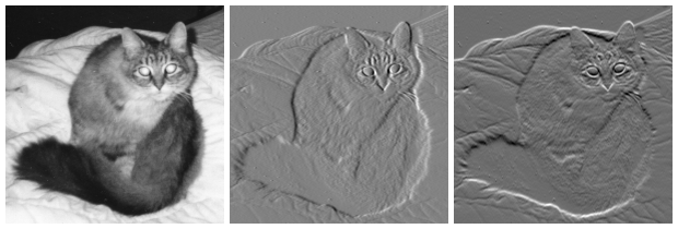(image courtesy to wiki)

On the left, an intensity image of a cat. In the center, a gradient image in the x-direction measuring a horizontal change in intensity. On the right, a gradient image in the y-direction measuring a vertical change in intensity.

• Apply non-maximum suppression: to get rid of spurious response to edge detection. So, after getting gradient magnitude and direction, a full scan of an image is done to remove any unwanted pixels which may not constitute the edge. For this, at every pixel, a pixel is checked if it is a local maximum in its neighborhood in the direction of the gradient.

• Apply double threshold: to determine potential edges.

• Track edge by hysteresis: Finalize the detection of edges by suppressing all the other edges that are weak and not connected to strong edges. For this, we need two threshold values, minVal and maxVal. Any edges with intensity gradient more than maxVal are sure to be edges and those below minVal are sure to be non-edges, so discarded. Those who lie between these two thresholds are classified as edges or non-edges based on their connectivity.

Resources:

• 1 - 2 - 3 - 4

Vectorization

Contour tracking

We can use a contour tracing algorithm to Scikit-Image to extract the paths around the object. This controls how accurately the path follows the original bitmap shape.

from sklearn.cluster import KMeans
import matplotlib.pyplot as plt
from skimage import measure
import numpy as np
import imageio

pic = imageio.imread('img/parrot.jpg')

h,w = pic.shape[:2]

im_small_long = pic.reshape((h * w, 3))
im_small_wide = im_small_long.reshape((h,w,3))

km = KMeans(n_clusters=2)
km.fit(im_small_long)

seg = np.asarray([(1 if i == 1 else 0)
                  for i in km.labels_]).reshape((h,w))

contours = measure.find_contours(seg, 0.5, fully_connected="high")
simplified_contours = [measure.approximate_polygon(c, tolerance=5) 
                       for c in contours]

plt.figure(figsize=(5,10))
for n, contour in enumerate(simplified_contours):
    plt.plot(contour[:, 1], contour[:, 0], linewidth=2)
    
    
plt.ylim(h,0)
plt.axes().set_aspect('equal')

Image Compression

Stacked Autoencoder

We like to conclude with a brief overview of Autoencoder. It’s a data compression algorithm where the compression and decompression functions are

• Data-specific,
• Lossy, and
• Learned automatically from examples rather than engineered by a human.

As it’s data specific and lossy, it’s not good for image compression in general. The fact that autoencoders are data-specific which makes them generally impractical for real-world data compression problems. But there’s a hope, future advances might change this. I find it interesting, though it’s not good enough and also very poor performance compared to another compression algorithm like JPEG, MPEG etc. Check out this keras blog post regarding on this issue.

And also some following stuff, in case if someone is interested too.

• 1 - 2 - 3

Now, I do realize that these topics are quite complex and lots of stuff can take concern and can be made in whole posts by each of them. In an effort to remain concise and complex free, I will implement the code but will skip explaining in details that what makes it happens and just showing the outcome of it.

import numpy as np
import matplotlib.pyplot as plt
import tensorflow as tf

from tensorflow.examples.tutorials.mnist import input_data
mnist = input_data.read_data_sets("MNIST_data",one_hot=True)

# Parameter
neurons_hid3    = neurons_hid1 # Decoder Begins
num_inputs      = 784 # 28*28
num_outputs     = num_inputs
learning_rate   = 0.01
neurons_hid1    = 392
neurons_hid2    = 196
num_epochs      = 5
batch_size      = 150
num_test_images = 10 # Test Autoencoder output on Test Data

# activation function
actf = tf.nn.relu

# place holder
X = tf.placeholder(tf.float32, shape=[None, num_inputs])

# Weights
initializer = tf.variance_scaling_initializer()
w1 = tf.Variable(initializer([num_inputs, neurons_hid1]), dtype=tf.float32)
w2 = tf.Variable(initializer([neurons_hid1, neurons_hid2]), dtype=tf.float32)
w3 = tf.Variable(initializer([neurons_hid2, neurons_hid3]), dtype=tf.float32)
w4 = tf.Variable(initializer([neurons_hid3, num_outputs]), dtype=tf.float32)

# Biases
b1 = tf.Variable(tf.zeros(neurons_hid1))
b2 = tf.Variable(tf.zeros(neurons_hid2))
b3 = tf.Variable(tf.zeros(neurons_hid3))
b4 = tf.Variable(tf.zeros(num_outputs))

# Activation Function and Layers
act_func = tf.nn.relu

hid_layer1   = act_func(tf.matmul(X, w1) + b1)
hid_layer2   = act_func(tf.matmul(hid_layer1, w2) + b2)
hid_layer3   = act_func(tf.matmul(hid_layer2, w3) + b3)
output_layer = tf.matmul(hid_layer3, w4) + b4

# Loss Function
loss = tf.reduce_mean(tf.square(output_layer - X))

# Optimizer
optimizer = tf.train.AdamOptimizer(learning_rate)
train     = optimizer.minimize(loss)

# Intialize Variables
init  = tf.global_variables_initializer()
saver = tf.train.Saver() 

with tf.Session() as sess:
    sess.run(init)
    
    # Epoch == Entire Training Set
    for epoch in range(num_epochs):
        num_batches = mnist.train.num_examples // batch_size
        
        # 150 batch size
        for iteration in range(num_batches):
            X_batch, y_batch = mnist.train.next_batch(batch_size)
            sess.run(train, feed_dict={X: X_batch})
            
        training_loss = loss.eval(feed_dict={X: X_batch})   
        print("Epoch {} Complete Training Loss: {}".format(epoch,training_loss))
    saver.save(sess, "./stacked_autoencoder.ckpt")       
    
with tf.Session() as sess:
    saver.restore(sess,"./stacked_autoencoder.ckpt")
    results = output_layer.eval(feed_dict={X:mnist.test.images[:num_test_images]})

Training phase; loss decreases with epochs.

Epoch (0,1,2,3,4) Complete Training Loss: (0.02334, 0.02253, 0.02003, 0.02132, 0.01938)

Let’s visualize some outcomes.

# Compare original images with their reconstructions
f, a = plt.subplots(2, 10, figsize=(20, 4))
for i in range(num_test_images):
    a[0][i].imshow(np.reshape(mnist.test.images[i], (28, 28)))
    a[1][i].imshow(np.reshape(results[i], (28, 28)))

Here, in the first row which is the loaded MNIST training set and the second row is the reconstructed those training set after encoding and decoding using autoencoder. Looks nice, but not great, there’s a lot of information missing in the reconstructed images. So, autoencoder is not as good as other compression technique but as a part of fast growing promising technology, future advances might change this, who knows.

At the ends of our 2 part series on Basic Image-Processing in Python, hope everyone was able to follow along, and if you feel that I have done something important mistake, please let me know in the comments!

Source Code: GitHub

Sources